Andorville™ Bayes Software
Introduction
The Andorville™ Bayes software is used to demonstrate and apply Bayes' theorem.
Bayes' theorem is used to update the probability of an event occurring when the result of a related event becomes known.
Bayes' theorem is also known as Bayes' law or Bayes' rule.
A Bayes model consists of two related events, Event A and Event B.
Event A is the condition we would like to determine, but the cost of determination is high.
For example, a colonoscopy could be used to detect bowel cancer, but the cost is over AUD$2,000 (in Australia in 2021).
Event B is a condition that is easy to determine, and the result is related to the probability of Event A.
For example, a fecal occult blood screen test costs about AUD$40 and produces a positive result in most cases where bowel cancer is present.
The screening test does however very often produce a positive result when no cancer is present (false positive) and sometimes a negative result when cancer is present (false negative).
Bayesian analysis is used to calculate the updated likelihood of a condition, such as bowel cancer, based on the result of a related event, such as a screening test.
The use of the Andorville™ Bayes software is demonstrated on this page using a bowel cancer screening test example.
The source code for the software can be downloaded from this GitHub page: ADVL_Bayes
Note that setup files are available on the GitHub pages but they are not code signed. Warning messages will appear when you run setup to install the software on a Windows 10 computer.
You can also open the source code in Visual Studio 2019 and run the software from there. The Visual Studio Community version is free to use.
Just click the "Clone a repository" option to copy the project from GitHub.
If you have any questions or comments, contact me at 
The data for the model shown in the demonstration is copied from the Wikipedia page:
Sensitivity and specificity
by wikipedia.org, text is available under the Creative Commons Attribution-ShareAlike License; additional terms may apply.
License text link: Text of Creative Commons Attribution-ShareAlike 3.0 Unported License
The example contains hypothetical bowel cancer screening test data.
The Bayes Application Main Form
The Main form contains the following tabs:
Workflow - The default workflow page contains a description of the application. Workflow pages are coded in HTML and can be edited by the user to provide a tailored user interface.
Bayesian Analysis - The Bayesian analysis page includes tools for data input and performance measures of events used for diagnostic testing.
Project Information - Information about the selected Andorville™ Bayes project. Projects contain information used by the application and can be linked together in a composite application.
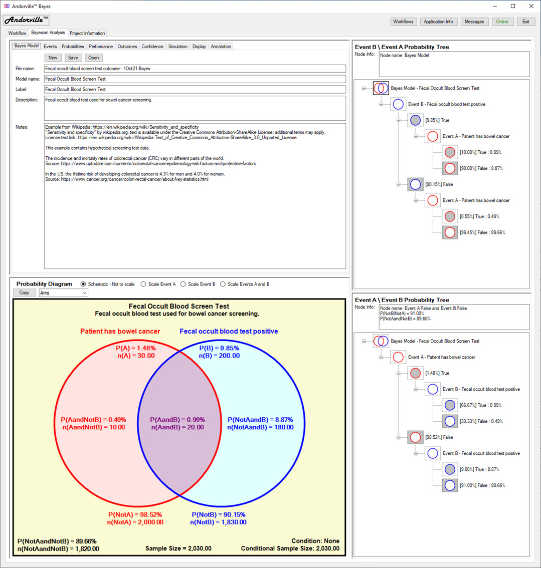
The Bayesian Analysis Tab
The Bayesian Analysis tab displays information about the Bayes model including survey sample counts and corresponding probabilities
for the two related events that comprise the Bayes model.
This tab is divided into four sections:
Model Information on the top left - shows information about the Bayes model on several tab pages, including the conditional probabilities and the diagnostic test performance of Event B.
Probability Diagram on the bottom left - shows a diagram of the two events that comprise the model and probabilities corresponding to event result combinations.
Event B \ Event A Probability Tree on the top right - shows the probabilities of an Event B result followed by an Event A result.
Event A \ Event B Probability Tree on the bottom right - shows the probabilities of an Event A result followed by an Event B result.
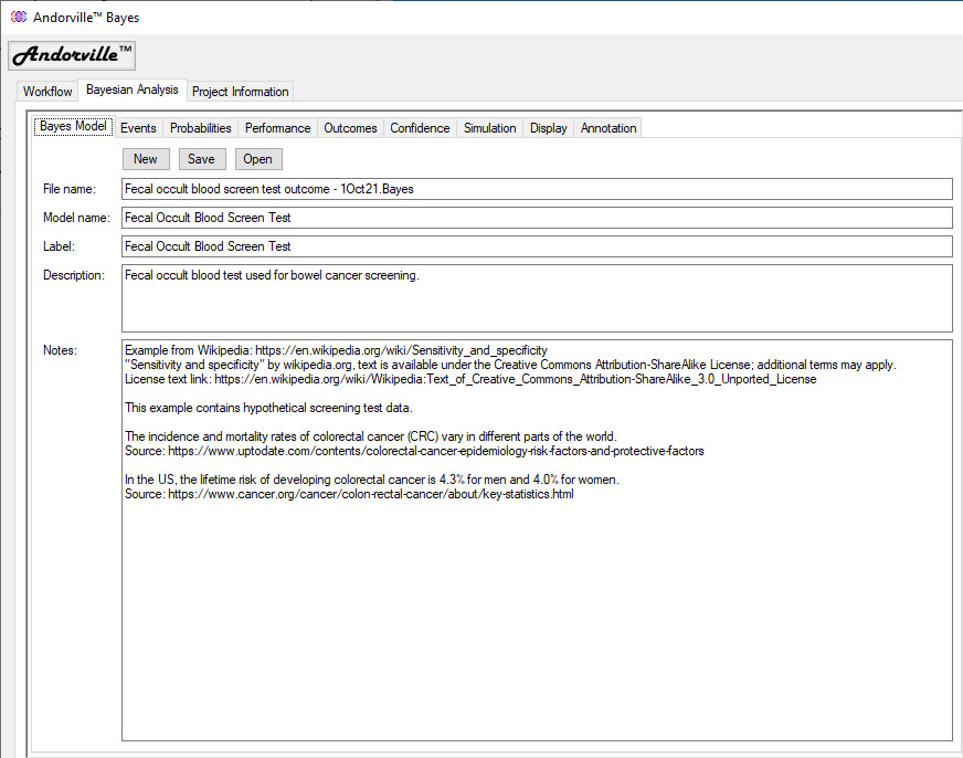
The Bayes Model Tab
The Bayes Model tab displays information about the selected model including the file name, model name, label, description and notes.
The label and description are displayed on the Probability Diagram.
An existing model can be opened and saved and a new model created from this tab.
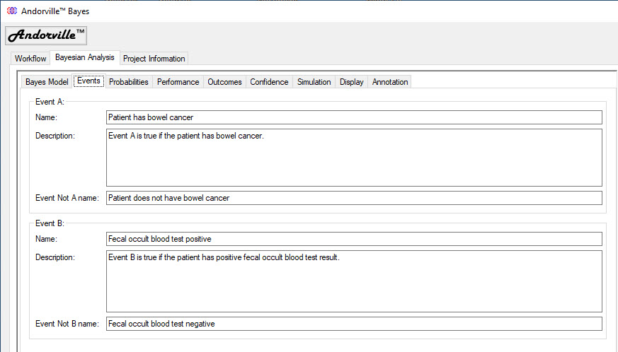
The Events Tab
The Events tab shows the name and description of each event.
In this example, the Event A name is "Patient has bowel cancer".
Names are also given to the Event False outcomes.
In this example, the name of Event A False (or Event Not A) is "Patient does not have bowel cancer".
The Probability Diagram
The Probability Diagram displays the Bayes model graphically.
Event A is drawn to the left as a red circle annotated with the Event A True label "Patient has bowel cancer".
Event B is drawn to the right as a blue circle annotated with the Event B True label "Fecal occult blood test positive".
The overlap area is shaded purple and represents the probability of Event A True and Event B True.
The overlap area represents the True Positive probability: the probability that the patient returned a positive screening test and has bowel cancer.
Probabilities are annotated using a capital P followed by the event result(s) in round brackets.
For example P(A) = 1.48% represents the probability of Event A True is 1.48%.
P(AandNotB) = 0.49% means that the probability of Event A True and Event B False is 0.49%.
Probabilities are usually calculated from survey counts and displaying the counts can help show how the probabilities are calculated.
Survey sample counts are annotated using a lower case n followed by the event result(s) in round brackets.
For example n(A) = 30 means that the number of times Event A True occurred in the survey was 30.
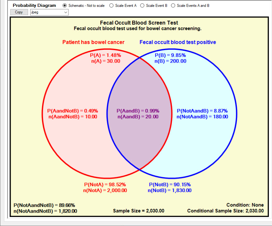
In the diagram above the event circles are drawn for clarity and are not to scale.
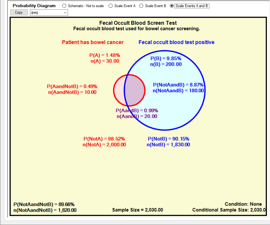
Four scaling options are available:
Schematic - Not to Scale - event circles are drawn for clarity and their sizes do not indicate the corresponding probabilities.
Scale Event A - Event circle A is scaled so that the area and overlap is proportional to the probability relative to Event B.
Scale Event B - Event circle B is scaled so that the area and overlap is proportional to the probability relative to Event A
Scale Events A and B - Event circles A and B are scaled so that the areas and overlap are proportional to the probabilities relative to the total diagram area.
The Scale Events A and B option has been selected in the Probability Diagram shown below.
The area of the red Event A circle is 1.48% of the total diagram area, scaled correctly to represent the 1.48% probability of Event A True.
The area of the blue Event B circle is 9.85% of the total diagram area, scaled correctly to represent the 9.85% probability of Event B True.
The overlap area is also scaled correctly to represent the 0.99% probability of Event A True and Event B True.
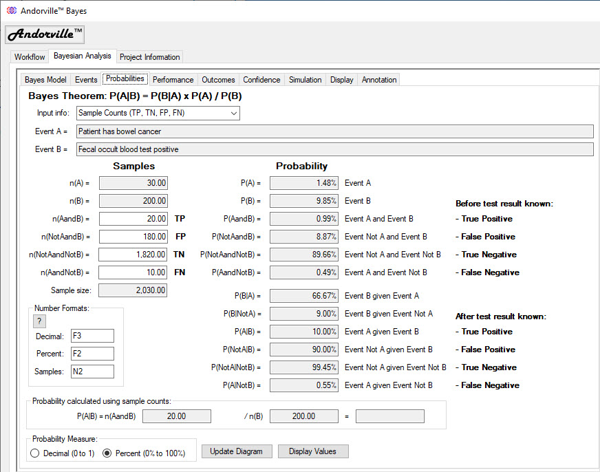
The Probabilities Tab
The Probabilities tab is used to enter known event probabilities or survey sample counts.
Remaining probabilities and sample counts are calculated from the input values.
Bayes theorem is used to calculate the probability of Event A True given Event B True.
This is usually expressed by the formula: P(A|B) = P(B|A) * P(A) / P(B)
where "Probability of Event A True Given Event B True" is represent symbolically as "P(A|B)".
This version of the formula assumes we know P(A), P(B) and P(B|A)
Any three independent probabilities and a survey sample size are required to specify a Bayes model.
Survey sample counts can also define a model.
In the example shown below, the survey sample counts for the true positives, true negatives, false positives and false negatives were entered.
This tab is also used to specify the display format for the sample count and probability values.
Probabilities can be displayed as decimal numbers or percentages.
Number format strings define exactly how the numbers are displayed.
Format string examples:
F4 - the number is displayed with 4 decimal places.
N4 - the number is displayed with thousands separators (,) and 4 decimal places.
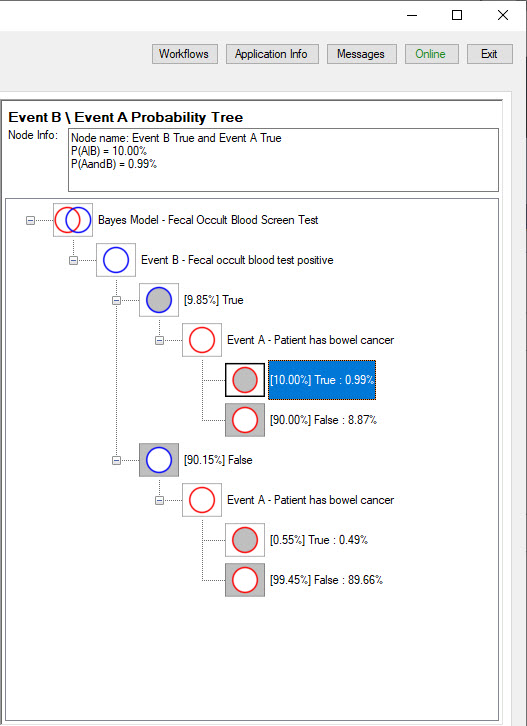
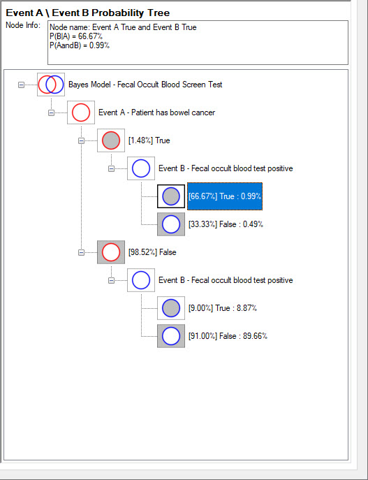
The Event B \ Event A Probability Tree
The Event B \ Event A Probability Tree shows the probabilities of an Event A result following an Event B result.
The probabilities in square brackets are conditional on the previous outcome.
The tree shows that the probability of Event B True is 9.85%. This is annotated on the third node down from the top.
Given Event B is True, the probability of Event A True is 10%. This is annotated on the selected node, the fifth node down.
Each pair of conditional probabilities, that branch from an event node, correspond to the two possible outcomes, True or False, and add up to 100%.
The four unconditional outcome probabilities are shown on final branch of each tree, without brackets.
These are the probabilities of each outcome before the result of Event B is known. These four unconditional probabilities add up to 100%.
In this example, if the screening test is positive (Event B True), the probability of cancer (Event A True) has been boosted (from 1.48%) to 10%
and further investigation is justified.
If the screening test is negative, the probability of cancer has been reduced to 0.55%.
The Event A \ Event B Probability Tree
The Event A \ Event B Probability Tree shows the probabilities of an Event B result given an Event A result.
In this example, we can see that if cancer is present (Event A True) the screening test will detect it with a probability of 66.67% (shown in square brackets).
If cancer is not present, the screening test will confirm this with a probability of 91.00%.
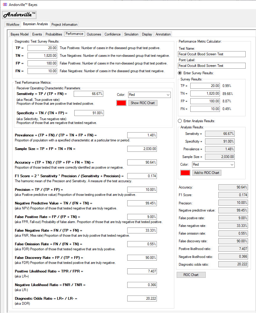
The Performance Tab
The Performance tab shows how well Event B performs as a diagnostic test for Event A.
The Diagnostic Test Survey Results shows the number of samples in each survey catagory of true positives (TP) true negatives (TN) false positives (FP) and false negatives (FN).
If these values were not entered they will be calculated using an assumed survey sample size.
The Test Performance Metrics section shows a range of commonly used performance measures.
The Sensitivity is the proportion of the population that are positive (have bowel cancer) that test positive (positive fecal occult blood test).
This parameter is also known as Recall and True Positive Rate.
The Specificity is the proportion of the population that are negative (do not have cancer) that test negative.
This parameter is also known as Selectivity and True Negative Rate.
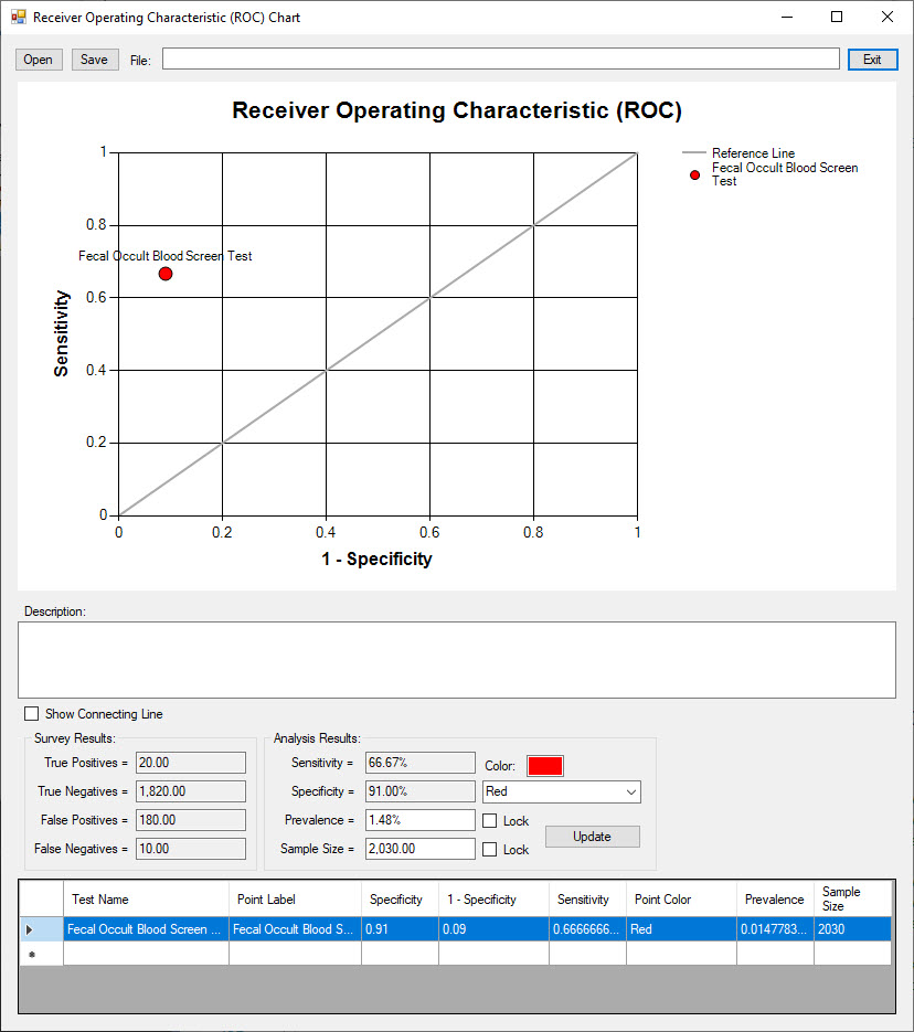
Cross-plotting Sensitivity against 1 - Specificity is often done to characterise the diagnostic test.
This cross-plot is called a Receiver Operating Characteristic (ROC) chart, named after its original use in measuring the performance of operators of military radar receivers.
Press the "Show ROC Chart" button to display the chart.
The Performance Metric Calculator section is used to calculate the metrics for any set of survey results or diagnostic test analysis results.
The Fecal Occult Blood Screen Test is plotted on the ROC chart below.
The Sensitivity (or True Positive Rate) is plotted along the Y axis.
1 - Specificity (or False Positive Rate) is plotted along the X axis.
A perfect diagnostic test would plot at the top left where Sensitivity = 1 and (1 - Specificity) = 0.
A diagnostic test plotting along the diagonal reference line would have no predictive value.
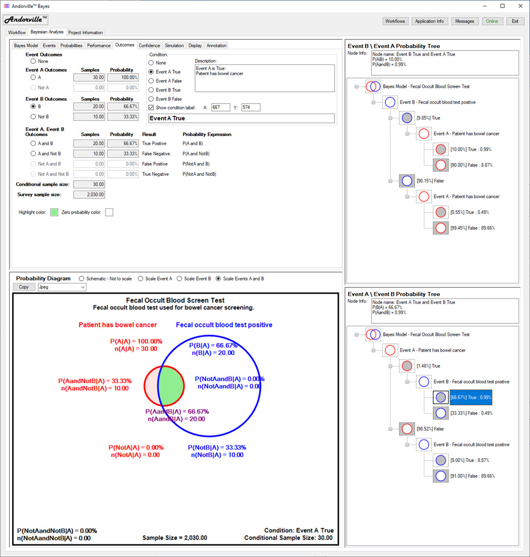
The Outcomes Tab
The Outcomes tab shows the list of possible outcomes and probabilities given specfied conditions.
This tab is linked to the probability trees and probability diagram.
When a node on a probability tree is selected, the outcome tab and probability diagram are updated.
In the example shown below, the "Event B True and Event A True" node has been selected on the Event B Probability Tree.
On the Outcomes tab, the corresponding "Event B True" Condition is selected and the probabilities of Event A True and Event A False (Not A True) are updated.
On the Probability Diagram, the area outside of the blue Event B circle, which now has a zero probability, is shaded in white, the zero probability color.
The selected Event B True and Event A True area is shaded in green, the highlight color.
The conditional probabilities and sample counts corresponding to Event B True are now annotated on the diagram.
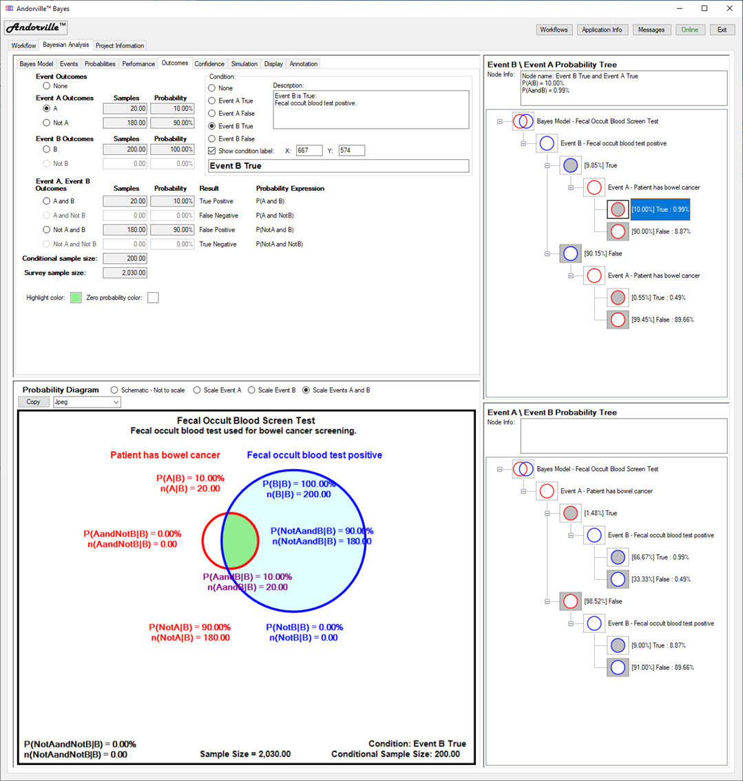
In the second example shown below, the "Event B True and Event A True" node has been selected on the Event A Probability Tree.
The "Event A True" condition is now selected on the Outcomes tab and the probabilities of Event B True and Event B False (Not B True) are updated.
On the Probability Diagram, the area outside the red Event A circle, which now has a zero probability, is shaded in white.
The selected Event B True and Event A True area is shaded in green, the highlight color.
The conditional probabilities and sample counts corresponding to Event A True are now annotated on the diagram.
While the result of Event B is usually determined before the result of Event A, this example shows the Sensitivity of the diagnostic test (Event B).
Sensitivity, also known as Recall and the True Positive Rate, is the proportion of those that are positive that test positive.
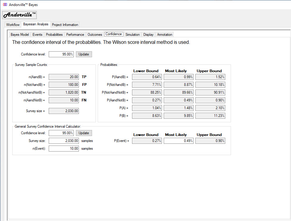
The Confidence Tab
The Confidence tab shows the confidence interval of the event probabilities estimated from survey data.
The most likely event probabilities are simply the survey event counts divided by the survey sample size.
The upper and lower probability bounds are calculated for a specified confidence level.
The Wilson score interval method is used to calculate the interval.
Low probability events are sampled relatively rarely in a survey and have wide confidence intervals relative to their most likely probability values.
Large sample sizes are needed to reduce the relative confidence interval of low probability events.
The Confidence tab includes a general survey confidence interval calculator.
The required confidence level, survey size and number of event samples are entered.
The most likely event probability and the upper and lower probability bounds are calculated.
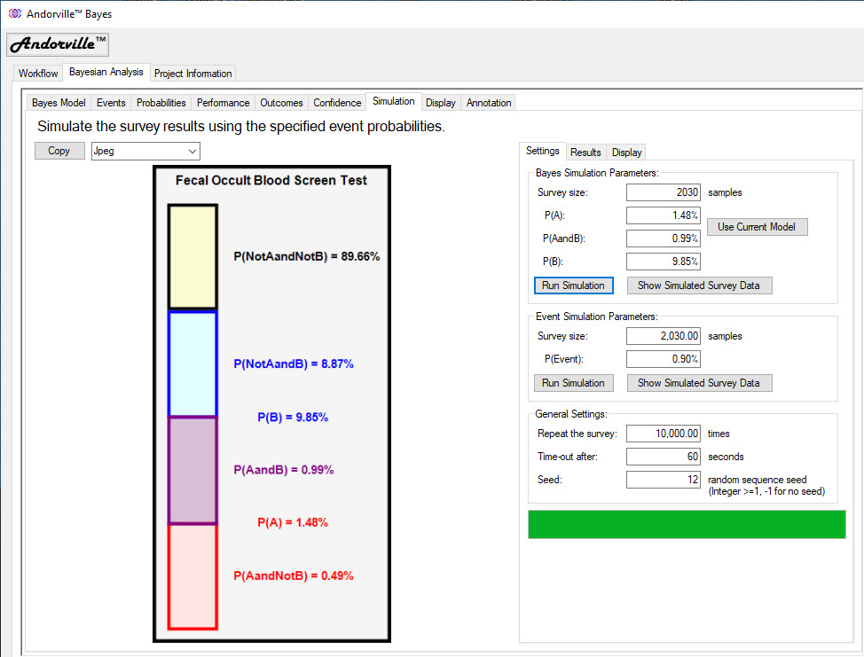
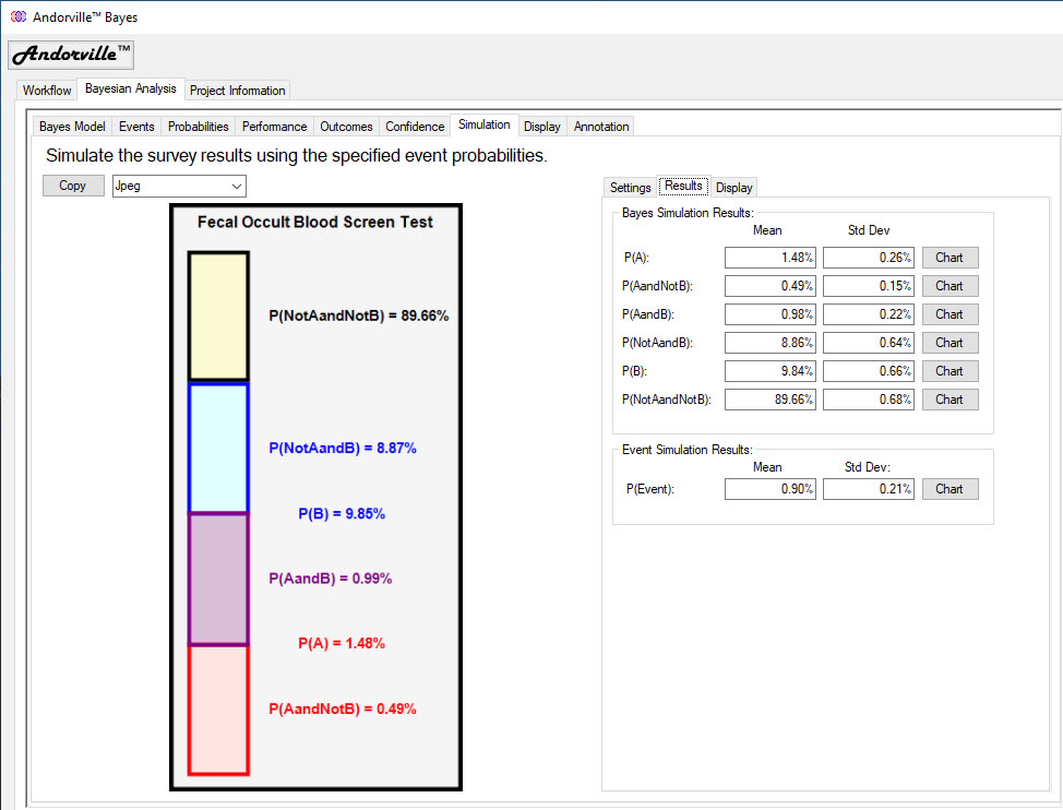
The Simulation Tab
The simulation tab is used to simulate a survey using exact assumed event probabilities.
The assumed probabilities and the survey size are entered in the Bayes Simulation Parameters section.
The P(A), P(AandB) and P(B) probabilities and the survey size define a Bayes model.
Press the "Use Current Model" button to use the values in the current model.
A simple bar chart is displayed to the left of the simulation settings.
This chart displays each event in the Bayes model with probability annotations.
The scaling of this chart is adjusted (from schematic to scaled) to match the scaling selected on the Probability Diagram.
The number of survey repeats is entered in the General Settings.
By repeating the simulated survey many times, a probability distribution of the number times each event will be sampled by the survey can be estimated.
The probability distributions can then be converted to distributions of the probability of each event as estimated by the survey. (This will be explained more clearly when the distribution charts are discussed.)
The General Settings includes a time-out setting that terminates the simulation if it has taken longer than the specified time.
A random sequence seed can be entered if a repeatable simulation is required.
Enter an integer greater than or equal to 1 to generate a repeatable simulation.
Enter a value of -1 for a new random simulation each time the simulation is run.
In the example shown below, the most likely event probabilities from the colon cancer screening model are used as the assumed known probabilities.
The model survey size is also used in the simulation.
The survey simulation is repeated 10,000 times to build up the event sampling distributions.
(On my computer it takes just a few seconds to run the 10,000 repeats.)
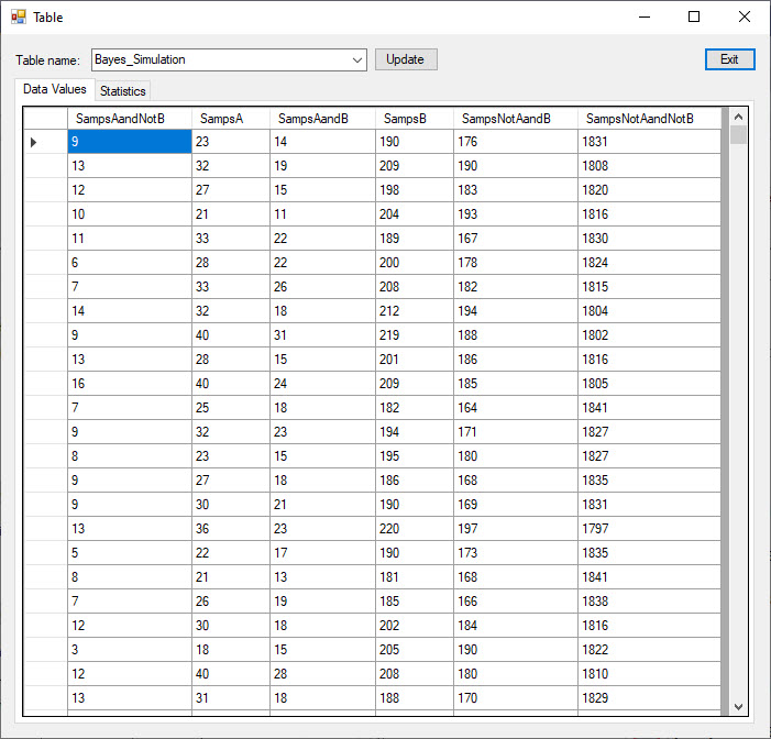
Pressing the "Show Simulated Survey Data" button displays the data table generated by the simulation.
The table contains 10,000 rows, one for each repeat of a survey simulation.
Each row shows the number of times different events were sampled during a survey.
There is some redundacy in these events: SampsA = SampsAandNotB + SampsAandB and SampsB = SampsAandB + SampsNotAandB
SampsAandB is the number of times Event A and Event B were sampled. This is the count of True Positives.
SampsNotAandB is the number of times Event Not A and Event B were sampled. This is the count of False Positives.
SampsNotAandNotB is the number of times Event Not A and Not B were sampled. This is the count of True Negatives.
SampsAandNotB is the number of times Event A and Event Not B were sampled. This is the count of False Negatives.
The highest probability event in this example is the True Negative, or SampsNotAandNotB, with a probability of 89.66% and 1,820 expected events in a survey size of 2,030 samples.
The data table shows event counts close to this value.
The lowest probability event is the False Negative, or SampsAandNotB, with a probability of 0.49% and 10 expected events in a survey size of 2,030 samples.
The data table shows a relatively wide variation of event counts about the expected count of 10.
The results of the simulation are summarised on the Results tab.
The mean and standard deviation of the sample counts are converted to probabilities by dividing by the survey size.
The event probability estimates produced by the surveys have mean values very close to the true values.
The standard deviation values indicate the variation in these probabilty estimates from survey to survey.
The nature of the variation can be displayed on a chart. Press the "Chart" button to the right of each event result to view the corresponding chart.
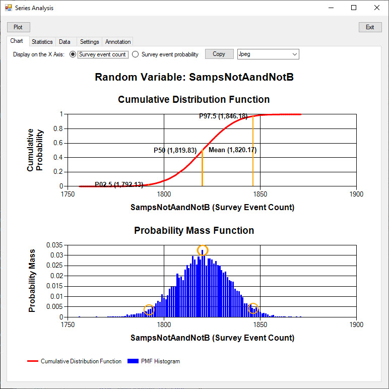
The Probability Mass Function displayed in the chart below shows the probability (Y axis) of each survey count of the event Not A and Not B (True Negative event).
The probabilities are estimated using the frequency of each count over the 10,000 repeats of the survey.
The mean event count of 1,820.17 is close to the 1,820 expected count.
The survey sampling process involving events having fixed probabilities is a Bernoulli process.
The corresponding Probability Mass Function (PMF) is a discrete probability distribution called a binomial distribution.
While the PMF values can be calculated using a formula, the size of the numbers used in the calculation become very large, and result in overflow errors, for even modest survey sizes.
In Excel a survey size larger than 170 trials produces overflow errors.
There are calculation methods involving approximations or logarithms that avoid the overflow issue.
(Excel's BINOM.DIST function uses such a method.)
The cumulative probability distribution shows the probability (Y axis) that a survey event count will be less than or equal to the X axis value.
The P02.5 and P97.5 cumulative probability values are annotated on this chart.
There is a 2.5% probability that the Not A and Not B event count in a survey will be less than or equal to 1,792.13.
There is a 97.5% probability that the Not A and Not B event count in a survey will be less than or equal to 1,846.18.
Taking the interval between these points, there is a 95% probability that the Not A and Not B event count will be between 1,792.13 and 1,846.18.
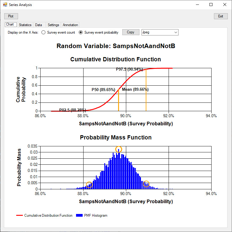
The Survey Counts along the X axis of the charts have been converted to probablities in the chart versions shown below.
The mean event probability is 89.66%, which is equal to the assumed event probability, to the 2 decimal places displayed.
The P50 value of 89.65% means that 50% of the time, a survey will produce a most likely (True Negative) event probability estimate less than or equal to 89.65%.
Because the P50 value is slightly smaller than the mean value, a slight amount of skew in the distribution is indicated.
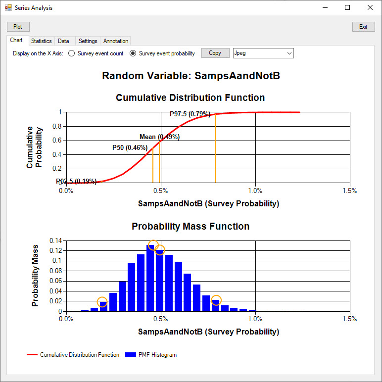
The Probability Mass Function of the False Negative survey probability is shown below.
This event has the relatively low mean probability of 0.49% and has a more skewed distribution that the higher probability events.
Using the 2,030 sample survey size, the event probability estimate from a single survey will lie between 0.19% (P02.5) and 0.79% (P97.5) with 95% confidence.
A larger survey size must be used if a more certain probability estimate is required.
The Simulation table includes the option to simulate a single event instead of a whole Bayesian model.
This can be used to determine if a specified survey size can be used to estimate the probability of an event with a specified probability to the required certainty.
This option can also be used to confirm the confidence intervals determined on the Confidence tab.
The 95% confident lower bound from the Confidence interval can used as the event probability in a simulation of the same survey size.
The P97.5 value (the upper bound of a 95% confidence interval) on the simulated probability distribution should be the same as the most likely probability on the Confidence tab.
A similar method can be used to confirm the upper bound of the confidence interval.
Conclusions
A Baysian model is fully defined using just four values.
These values can consist of either three independent probability values and a survey sample size, or four survey counts: the number of true positives, true negatives, false positives and false negatives.
From those few numbers we can determine many useful properties about the underlying two related events, including:
- how well Event B performs as a diagnostic test for Event A
- the prevalence of Event A
- generate a total of 40 conditional and unconditional probabilities (including trivial values)
- generate a total of 40 conditional and unconditional sample counts
- the confidence interval of most likely probabilities determined using sample counts.
The Andorville™ Bayes software is a useful tool for defining, analysing and understanding a Bayes model.
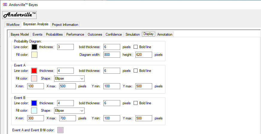
Appendix 1 - The Display Tab
The Display tab is used to define the display settings for the Probability Diagram.
The size, color and position of the Event A and Event B circles in the schematic scaling can be adjusted.
The shading color of the key probability areas can also be set.
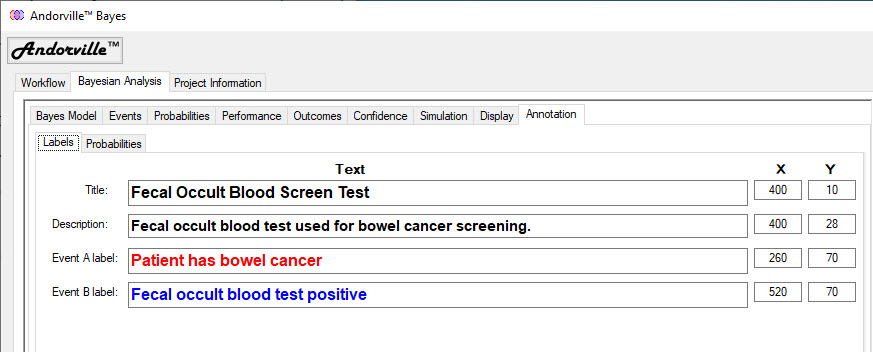
Appendix 2 - The Annotation Tab
The annotation tab is used to set the color, font and position of the annotations displayed on the Probability Diagram.
The Labels tab, shown below, adjusts the settings for the diagram title and description and the Event A and Event B titles.
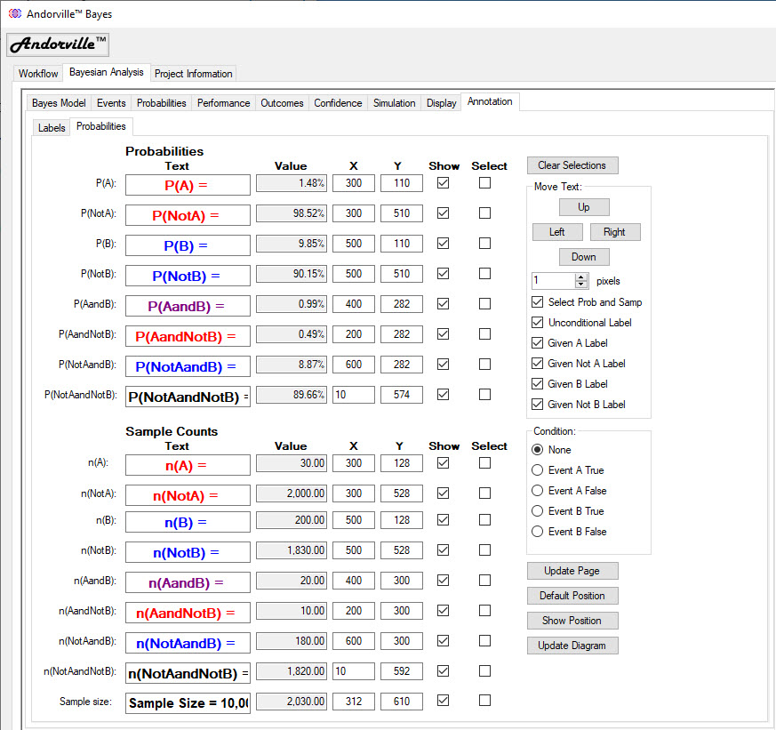
The Probabilities tab, shown below, adjusts the settings for the probability and sample count labels.
The label properties can change with the conditional probabilities and with the scaling selected.