This example shows how oil and gas exploration and production companies estimate the recoverable volumes of oil and gas trapped in geological structures two kilometres or more underground.
The volume of recoverable gas depends on many input values including the volume of rock containing the gas, the porosity and permeability of the rock and the properties of the gas.
These input values are estimated using seismic data to detect the depth and shape of the geological structure and well intersections to sample the rock and gas properties within the structure.
The input values are not known exactly but probability distributions can be defined using the available data.
Triangular distributions are often used for simple but adequate models.
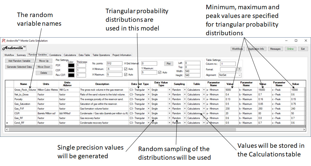
In this example the gas resource estimation random variables are defined as:
| Name | Distribution | Units | Min | Max | Peak |
|---|---|---|---|---|---|
| Gross Rock Volume | Triangular | Million Cubic Metres | 5000 | 15000 | 10000 |
| Net to Gross | Triangular | Factor | 0.4 | 0.7 | 0.6 |
| Porosity | Triangular | Factor | 0.13 | 0.16 | 0.15 |
| Gas Saturation | Triangular | Factor | 0.5 | 0.85 | 0.75 |
| Gas Volume Factor | Triangular | Factor | 230 | 250 | 240 |
| Condensate Ratio | Triangular | bbl/MMscf | 20 | 80 | 50 |
| Gas Recovery Factor | Triangular | Factor | 0.6 | 0.8 | 0.7 |
| Condensate RF | Triangular | Factor | 0.5 | 0.7 | 0.6 |
Triangular probability distributions can be used for simple models.
Other distributions may be used for more refined models.
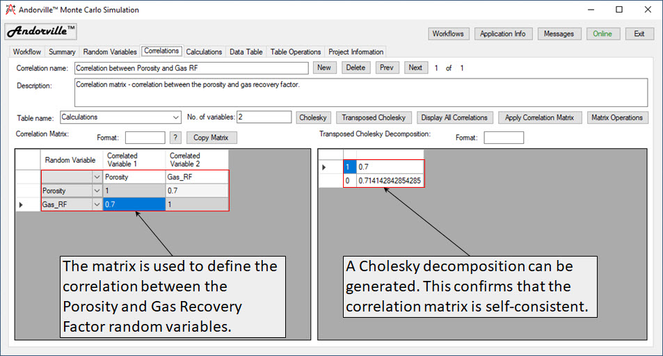
A correlation matrix is used to specify the correlation factors between random variables.
A correlation coefficient of 0.7 is defined between the Porosity and Gas Recovery Factor variables.
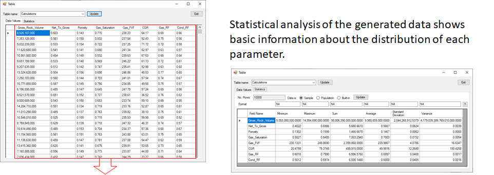
The Monte Carlo software generates reservoir rock and gas property values for the specified number of trials.
10,000 trials were run in this example.
Some of these values are shown in the table below.
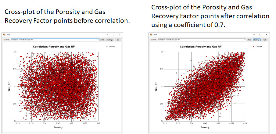
Gas recovery factors tend to be correlated to the rock porosity.
Reservoir simulations and experience provide a guide to suitable correlation coefficients.
A coefficient of 0.7 is used in this example.
More refined models will define correlations between other random variables.
A calculation tree is defined to read the reservoir and gas properties from the table, perform calculations for gas in place and recoverable gas then write these calculated values back to the table.
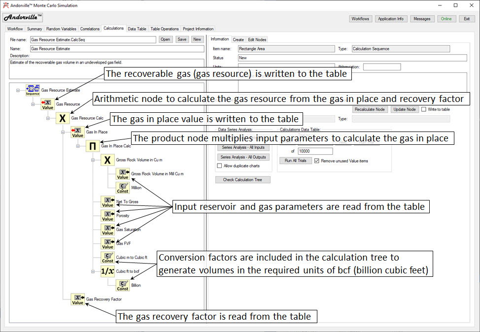
The Monte Carlo software generates the specified calculated values for the number of trials used in the model.
In this model, the Gas In Place and Gas Resource volumes are calculated.
This completes the simulation.
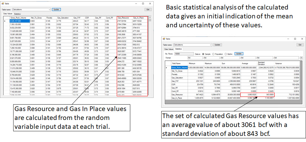
Some of calculated volumes are shown in the table below.
The cumulative probability and probability density charts shown below show the simulated Gas Resource probability distribution graphically.
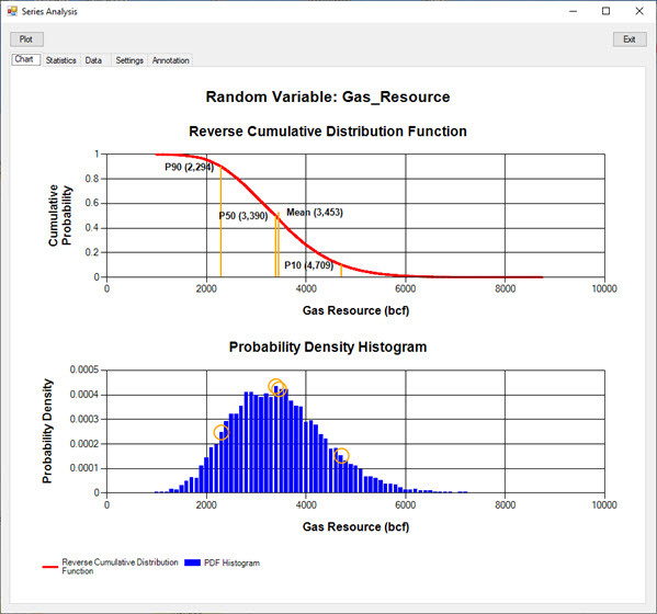
The Monte Carlo simulation shows that the calculated gas resource volume has a mean value of 3,453 billion cubic feet (bcf).
Reverse cumulative distribution functions are used to display resource volume distributions. The P90 value of 2,294 bcf means the gas
resource volume has a 90 percent chance of being 2,294 bcf or larger.
Resource development companies usually require the P90 volumes to be profitable before proceeding with the cost of a development project.